Overview
I developed a technique to render single-pixel particles (using additive blending) with compute shaders rather than the usual fixed-function rasterization with vertex and fragment shaders. My approach runs 31–350% faster than rasterization on the cases I tested and is particularly faster for some “pathological” cases (which for my application are not actually that uncommon). I observed these speedups on both NVIDIA and AMD GPUs.
Using this technique allowed me to ship an app that runs on minimum-spec hardware without sacrificing visual fidelity.
(UPDATE: After posting this article, I discovered that I could use the NV_shader_atomic_int64 OpenGL extension (which is also supported by newer AMD GPUs). With this extension my results are now 37–432% faster than rasterization on the cases tested. I recommend using it where possible. See the Addendum for more information.)
Background and Motivation
I developed a custom engine for the VR app I wrote over the course of 2 years: PARTICULATE. The app enables the user to create interesting particle effects and scenes, so the particles take the front seat, and the vast majority of GPU time is spent on simulating and rendering them. (Note that I do all particle simulation on the GPU as is common these days.)
The trailer for the app gives a feel for the particle rendering it does:
The app needs to render 2 million+ particles to two framebuffers (one for each VR eye) at 90hz. All particles are rendered using additive blending, so no sorting is necessary before rendering.
There are three types of particles that are rendered: two types are larger, velocity-stretched particles (of which there are at most a few tens of thousands). Rendering time is dominated by the third type, which comprises the smallest particles (of which there are millions).
For the rest of this article, when I refer to “particles” I am talking about these smallest particles. The larger ones (which are part of the same “particle cloud”) are rendered using velocity stretched quads in a geometry shader, and take up a minuscule amount of rendering time because there are comparatively few of them.
Speeding Up the Rasterization-based Approach
I was originally rendering the smallest particles as point sprites. The size of point sprites is never smaller than a pixel, so I would proportionally darken them if their projected on-screen size was actually less than 1 pixel. (The technique to find a particle’s projected on-screen size for an asymmetric projection matrix is described here.) As a side-note, this 1-pixel clamping / darkening is a good way of avoiding geometric aliasing for the particles as well.
Performance was not good enough for minimum-spec GPUs (NVIDIA GTX 970 and AMD R9 290), and particle rendering was the biggest expense, so I needed to speed it up. Since overdraw is usually a big culprit for particle rendering, I first experimented with reducing particle sizes (smaller quads with a steeper falloff texture). As expected this did improve performance, but it was still not good enough in a number of common cases.
Initially as an experiment, I then tried clamping particle size to 1 pixel (so in addition to particles never being smaller than a pixel, they could also never be larger than one). In the same way that particles are proportionally darkened when their projected size is smaller than a pixel, they are proportionally brightened when their projected size is larger than a pixel.
Unsurprisingly this was a performance win—but surprisingly it was also a quality win! In VR screen resolution is at a premium, so any finer grained detail is very noticeable, and the lack of a perspective effect on the on-screen size of particles wasn’t noticeable because with millions of small, dim particles (that are usually in motion) one tends to observe the shapes formed by the particles rather than each one individually.
Pathological Cases Motivate Trying Something Different
At this point, performance was usually good enough, but there were certain pathological cases, where the same number of on-screen particles would take much longer to render. (And these cases are unavoidable in my app because the user has full control over the forces affecting particles and thus their configuration—and these cases are not actually that uncommon, either.)
I noticed that, on NVIDIA hardware in particular (I was using a GTX 980), if the particles were spread relatively evenly across screen space OR if they were clumped up to very small screenspace regions (like thousands of particles rendered to just a few pixels) performance would tank. In more-average situations—the particles don’t spread across the whole screen but are also not super-clumped—performance was acceptable.
To give an idea, rendering time could vary by more than 3x for the same number of on-screen particles depending on their on-screen configuration (and remember that particles are always rendered as a single pixel, so this wasn’t a proximity-based fill rate issue).
I’m not sure what causes these discrepancies, but it’s likely due to details in the low-level implementation of the rasterization pipeline (and of course that differs on NVIDIA vs. AMD GPUs, and between generations of GPUs by the same vendor, etc.).
At this point, I decided to experiment with skipping fixed-function rasterization entirely and rendering the particles using compute. This makes a lot of sense in my case because:
- No actual rasterization is happening when rendering single-pixel particles—fundamentally we’re just splatting single pixels to the screen.
- Rasterization requires that 2x2 quads be executed even when rendering triangles that cover just a single pixel. This is very wasteful of occupancy and also totally unnecessary in my case as I do not rely on screenspace derivatives.
- Rendering APIs guarantee that primitives are drawn in the order they’re given, but this is unnecessary when additive blending is used (which it is for my particle rendering). This constraint could potentially be costing performance.
Developing the Compute Shader Rendering Technique
I’m not going to describe everything I tried here, but I do want to give the broad strokes explanation of how I arrived at the technique I’m using as this context explains the choices I made.
In order to render with a compute shader, we need either to sort particles by output pixel (or screenspace tile) so that each output pixel is written to by at most one thread, OR we need to update output pixels atomically so that writes from multiple threads don’t conflict.
I did look into tiled rendering (particularly the approach to tiled particle rendering outlined in this presentation by Gareth Thomas) but decided that it is not a good fit for my case. As far as I can tell, tiled rendering won’t work well for my app because particles may be (and often are) very “clumpy” in screenspace, which would cause massive imbalances in the amount of work needed for some tiles. (It’s possible, for example, for every single particle to be contained in just a few screenspace tiles). Thus parallelism would be very low, and worst-case performance would be very bad.
Light tiling (or clustering) approaches generally rely on a relatively even (or at least not massively uneven) distribution of lights across the grid being tiled. The presentation by Thomas I mentioned above also relies on this, and it shows benchmarks for scenes where particles are fairly spread out in screenspace.
So I decided instead to go down the road of updating pixel colors atomically. This approach allows me to avoid binning particles into screenspace tiles and the resulting imbalances doing so can cause.
Additive Blending Using Atomic Operations
There are a few challenges with updating pixel colors atomically via a compute shader. (I should note here that my engine uses OpenGL (4.5) as its rendering backend, so I am constrained by what’s possible in that API.) I’m using RGBA half-float (16 bit) textures for my framebuffers (for HDR rendering, which is important for additive blending of particles), and there is no way to atomically add to a half-float in OpenGL. (I’m guessing this is the case in other APIs as well, though I haven’t confirmed that.)
OpenGL also doesn’t support atomic adds to full (32-bit) floats, though there is an NVIDIA extension that enables this. However, as far as I know there is no equivalent AMD extension, and also (as I’ll discuss later) I can’t afford performance-wise to update 3 full floats (one for each color channel) for every particle
Thus I was forced down the road of using integer values to represent color channels, as those are what can be added to atomically in a compute shader. This unfortunately complicates things, as it means the rendering compute shader needs to update a separate buffer (not the normal framebuffer) and then composite the result back onto the normal framebuffer. And because the compute shader needs to operate on integers, it needs to translate particle colors from float to integer when doing the atomic adds and then translate the result back to float when compositing.
There are two things to determine, then:
- How to convert between float and integer color channel values.
- The bit depth of the RGB integer colors channel value that are added to for each particle.
Because the color channels are HDR (meaning they aren’t clamped to [0,1]), the conversion process isn’t as simple as what is normally done for 8-bit normalized channels, say (which are clamped to [0,1]). And because we’re doing atomic adds to the channels, they need to be represented in linear space, so no nonlinear tricks like sRGB can be used to conserve bits of precision.
I settled on converting HDR float values to integer ones through the following process. First empirically determine the maximum value a channel (for a pixel) can have after summing the contributions of every particle. Note that I say “empirically” here because this doesn’t have to be the theoretical maximum value (but rather a “likely” maximum for my application), and in fact if integer overflow happens occasionally it’s not the end of the world (as I’ll elaborate on later). Call this empirical maximum \( E_{\text{max}} \).
Call the maximum storable unsigned integer value \( I_{\text{max}} \). (This is dependent on the integer bit depth that is used to represent each channel—more on that next.) We can then convert a float color value \( c_{\text{f}} \) to an (unsigned) integer one \( c_{\text{i}} \) using the formula
\[ c_{\text{i}} = \text{round}(c_{\text{f}} \cdot \frac{I_{\text{max}}}{E_{\text{max}}}) \]This spreads the expected float range across the available integer range.
The most obvious way to proceed would be to allocate 3 uints per pixel for the 3 color channels and atomically add to each of them for every particle. I tried this, and it was too slow. Luckily, we can pack multiple color channels into a single uint. For example, the 3 color channels can be packed into a 32-bit uint by allocating 11 bits for R, 11 bits for G, and 10 for B (call this R11G11B10). Then we can atomically add all 3 at once using a single atomicAdd operation.
There is one caveat to this, which is that this means the high bits for one channel can overflow into the low bits of another—in the R11G11B10 case, G can overflow into R and B can overflow into G. Assuming the \( E_{\text{max}} \) above was chosen well, however, this is unlikely to happen (and when it does happen it is often unnoticeable as will be explained later).
I did try the R11G11B10 approach (which uses a single uint per pixel), and it did not work well. There are far too few bits per channel to handle the dynamic range that I am working with—individual particles can be very dark (especially when positioned far from the viewer, as they are darkened with distance), but thousands of them can add together to HDR values as high as 10.0. When I tried this approach, there were very noticeable color shifting effects due to precision as the viewpoint (and particles) moved around.
So 1 uint per pixel was too little (for precision reasons), and 3 was too much (for performance reasons). This left me to try packing the 3 color channels into 2 uints. Things were getting complicated, but I knew I was close, and I was determined to make this work :)
(NOTE: See the Addendum for a simpler (and faster) approach that can be used when the NV_shader_atomic_int64 OpenGL extension is available.)
I ended up settling on the following approach. The 3 channels are divided among the combined 64 bits of 2 uints. R and B are both allocated 21 bits in one of the 2 uints, and G is allocated 22 bits that are split across the 2 uints. So the first uint is R21Gh11 (‘Gh11’ is the high 11 bits of G) and the second is Gl11B21 (‘Gl11’ is the low 11 bits of G).

The RGB color channels are packed into two 32-bit uints: R21Gh11 and Gl11B21. The 22-bit G channel is split in half—its high 11 bits (Gh11) are in the first uint, and its low 11 bits (Gl11) are in the second.
There is an obvious complication here, which is that because G is split across the 2 uints, overflows when adding to the low 11 bits of G will be lost and not carried to the high 11 bits. The solution to this is to check if this overflow happened after the atomicAdd to Gl11B21. We can do this by using the return value of atomicAdd(), which is the value prior to the atomic addition. We take this return value, unpack Gl11 from it, and then add the Gl11 value that was added in the atomicAdd call—and then test if this addition overflowed the 11 bits. If it did overflow, we then add the overflowed bit(s) (right-shift the result of the addition by 11) to Gh11 in the other uint.
It’s fine that the second atomicAdd is non-atomic with the first, as the order of additions to each uint is not important (we just want to guarantee that the carried bit(s) are not lost). There is shader code later in this article showing exactly how this is done.
Everything Else Done by the Compute Shader
So far I’ve only described how the additive blending works in the compute shader. There are a few other things it does. (These are a subset of the things that would happen in normal rasterization.)
First it culls particles that are outside the view frustum. This is easy, as particles are always a single pixel, so no clipping is required. Then it computes screenspace coordinates and does the depth test. (Particles don’t write to the depth buffer, but earlier rendering does.) The fragment color is computed using the per-particle color scaled by projected area in screenspace divided by 1 pixel (the actual area), as described earlier. Then the additive blending happens as just described.
This is the shader code that converts a particle’s world-space position to a pixel coordinate in screenspace:
vec4 clipSpacePosition = u_matWVP * vec4(worldPosition, 1.0);

// Frustum cull before perspective divide by checking of any of xyz are outside [-w, w].
if (any(greaterThan(abs(clipSpacePosition.xyz), vec3(abs(clipSpacePosition.w))))) {
	return;
}

vec3 ndcPosition = clipSpacePosition.xyz / clipSpacePosition.w;
vec3 unscaledWindowCoords = 0.5 * ndcPosition + vec3(0.5);

// Technically this calculation should use the values set for glDepthRange and glViewport.
vec3 windowCoords = vec3(u_renderTextureDimensions * unscaledWindowCoords.xy,
	                     unscaledWindowCoords.z);

// Account for pixel centers being halfway between integers.
ivec2 pixelCoord = clamp(ivec2(round(windowCoords.xy - vec2(0.5))),
                         ivec2(0), u_renderTextureDimensions - ivec2(1));
In order to not tank performance, I needed to build a hierarchical depth buffer to use for coarse depth tests. In the general case, this requires generating the full mip chain from the full-res depth buffer (where the value of a texel at level N is equal to the min of the 4 texels it subsumes from level N-1). However, in my case I only query one mip level (level 4, or 1/16th x 1/16th resolution), so I am able to use a fast single-dispatch compute shader that generates just this one level. (See my article on hierarchical depth buffers for a detailed explanation of this approach.)
The depth test in the rendering compute shader queries the depth in the reduced-res depth buffer first, and then only the full-res buffer when necessary. I do this to have a fast out for the common case that a particle is in front of opaque geometry, thus reducing memory pressure for depth tests. This is similar to the Hi-Z optimization in some GPUs. I suspect that always testing against the full-res depth buffer was tanking performance because the accesses were effectively random (as I’m not tiling or sorting particles in any way).
So in summary, the basic idea of the approach I took is to allocate a new buffer with 2 uints per pixel, clear that buffer to 0’s every frame, and then run the compute shader described above to determine the pixel location of each particle (as well as its color), convert that color to uint, and do atomicAdd’s on the 2 uints corresponding to that pixel. Then do a full-screen triangle pass that reads the final uint values, converts them back to float, and additively blends them onto the normal framebuffer.
Performance Comparison
I compared the performance of using the normal rasterization pipeline (with single-pixel point sprites) to the compute shader rendering technique I just described. For the comparison I rendered the following three exact images. All are of scenes containing approximately 2 million particles. The images are 1648x1776, which was the eye buffer resolution requested by the Oculus SDK. Note that I’m measuring VR rendering performance, so in reality two eye buffers were rendered to—I’m only showing the left eye here.
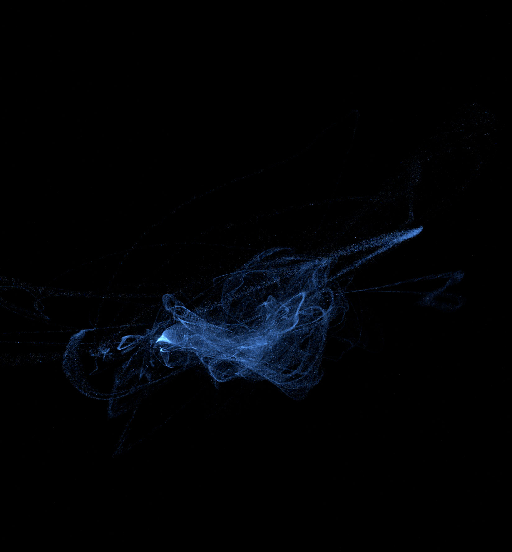
‘normal’ — This is a fairly representative image as far as normal app performance goes (particles are not normally covering the entire screen).
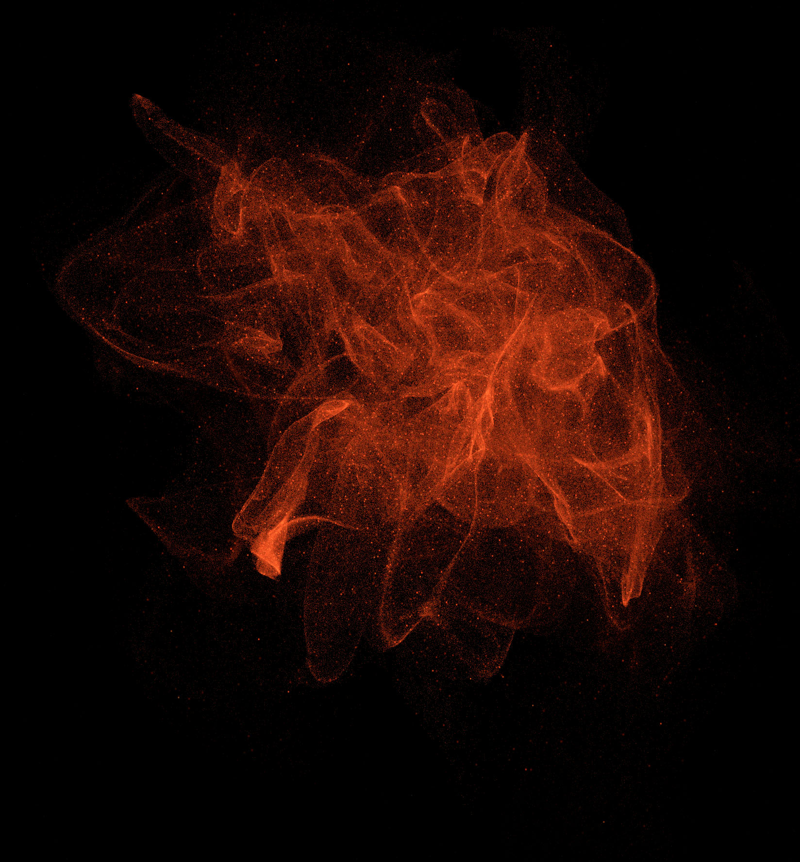
‘spread’ — Here particles are spread out across the rendered image. This case was resulting in large slowdowns when using rasterization.
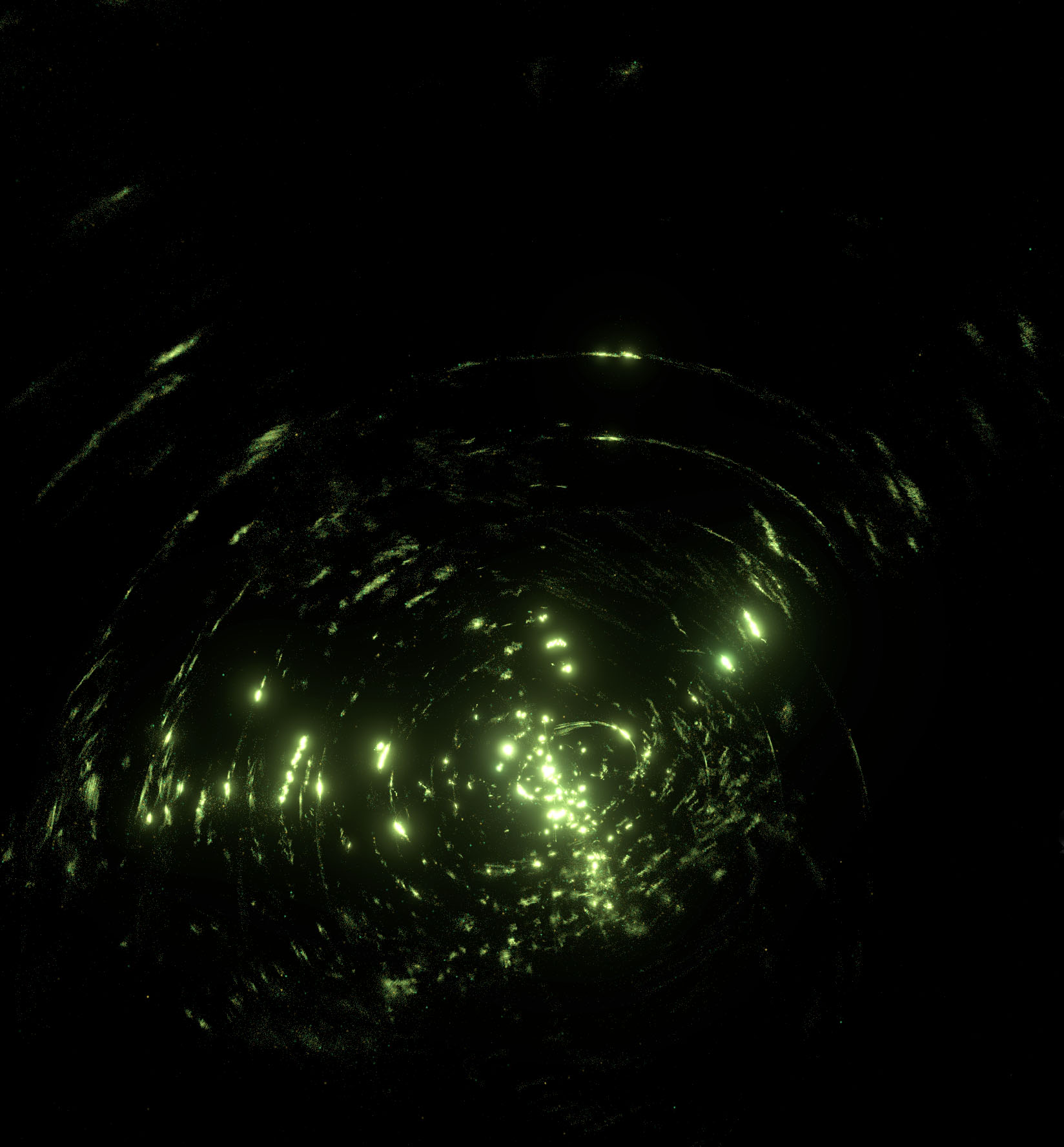
‘clumpy’ — Here particles are clumped together into very small on-screen regions (post-process bloom is causing these regions to expand in the final image). This case was also resulting in large slowdowns when using rasterization.
These were the results for rendering the particles to the two eye buffers for each of the above test cases on an NVIDIA GTX 980:
| ‘normal’ | ‘spread’ | ‘clumpy’ | |
|---|---|---|---|
| Rasterization | 4.2 ms | 11.1 ms | 11.7 ms |
| Compute shader | 2.3 ms | 6.1 ms | 2.6 ms |
| % change | -45% | -45% | -78% |
And these were the results for an AMD R9 290:
| ‘normal’ | ‘spread’ | ‘clumpy’ | |
|---|---|---|---|
| Rasterization | 3.7 ms | 5.9 ms | 3.1 ms |
| Compute shader | 2.2 ms | 4.5 ms | 2.2 ms |
| % change | -41% | -24% | -29% |
(Note that in this comparison I’m including all the additional costs of the compute-shader-based rendering approach, including clearing and compositing the uint buffer each frame, as well as generating the reduced-res depth buffer (so I’m assuming the latter isn’t already available for some other purpose).)
As we can see from the tables, compute shader rendering is a significant improvement for all three test cases on both the NVIDIA and AMD GPUs. The biggest improvement is for the ‘clumpy’ image on NVIDIA (-78% rendering time, or 350% faster). Given how poorly rasterization performed for that case vs. both NVIDIA with compute shader rendering and AMD with both types of rendering, I’m guessing there is something pathological going on for that case on the NVIDIA hardware tested.
The AMD GPU shows significant—though less dramatic—improvements. It’s also interesting that the AMD R9 290 performs better than the NVIDIA GTX 980 on every test (both using rasterization and the compute shader approach) given that the 290 is a less powerful GPU than the 980 overall.
Additional Details
Integer Quantization Error
I mentioned earlier that I initially tried packing the bits for all three color channels into a single 32-bit uint. This didn’t work because the quantization was too coarse, resulting in very noticeable color shifting as the distance between the particles and the viewer shifted (as particle colors are scaled in proportion to what their projected on-screen area would be).
Precision is much higher with the approach I took, but some color shifting effects are still visible at very far distances. In these cases, the colors of individual particles are getting scaled to very small values, so relative error for the color of each particle becomes much higher (and then this error is magnified as many particles are summed together). In practice this isn’t an issue in my app, as the user is never far enough away that these effects are visible.
If it were necessary to view particles at large distances, it would probably be possible to use an LOD scheme: render fewer particles with distance and proportionally brighten the ones that are rendered to account for the ones that aren’t. This way the quantization error for individual particles could be held constant rather than increasing with distance.
Color Channel Overflow
Earlier I mentioned that integer overflow is possible for the color channels when summing the contribution of each particle. When overflow happens for a channel, that channel’s value wraps around to zero, and an adjacent channel can have spurious bits carried over to it (e.g., the high bits of B can overflow into the low bits of G). This will not happen often if \( E_{\text{max}} \) is chosen well. \( E_{\text{max}} \) is the floating point value corresponding to the maximum representable integer value—if it’s too high, quantization of individual particles will be too coarse, and if it’s too low, overflow will happen too often.
For the value of \( E_{\text{max}} \) used in my app, there is sometimes overflow, but it isn’t visible. This is because only small regions of the hottest pixels will overflow (if any pixels overflow at all), and because of the post-process bloom effect applied later, nearby bright pixels (that themselves didn’t overflow) will bloom over and obscure the overflowed pixels.
atomicAdd Dependencies
Earlier I detailed how the two per-pixel uints are atomically added to for each particle. I capture overflows to the low bits of the G channel (in one uint) and add those to the high bits of the G channel (in the other uint).
My initial approach to this was to always perform two atomicAdd’s: First add to the uint containing the low bits of G. Then when that returns, test if there was overflow and add to the second uint (containing the high bits of G) incorporating the carried bits.
It turns out that doing the atomicAdd’s this way is substantially slower (on the NVIDIA hardware I tested, at least) than simply adding to the two uints in a non-dependent fashion. I haven’t looked into this in more detail, but I suspect that the two atomicAdd’s can be parallelized, but this can’t happen when the second atomicAdd depends on the result of the first.
The approach I ended up using first does independent atomicAdd’s to both uints. It then tests if the low bits of G overflowed for the uint that contains them. If they did, it performs a third atomicAdd to the uint containing the high bits of G to carry the overflowed bits. Because this carry is needed very rarely, this is only marginally slower than doing two independent atomicAdd’s (which is to say, better than the dependent approach I tried initially).
This is the shader code I use to pack the color channel values and perform the (up to three) atomicAdd’s:
// RG uint contains R in the high 21 bits and the high 11 bits of G in the low 11 bits.
uint rgValueToAdd = ((fragmentColorAsUint.r << 11) | (fragmentColorAsUint.g >> 11));

// GB uint contains the low 11 bits of G in the high 11 bits and B in the low 21 bits.
uint gbValueToAdd = ((fragmentColorAsUint.g << 21) | fragmentColorAsUint.b);

atomicAdd(perPixelRGBAtomicUints[rgUintIndex], rgValueToAdd);
uint previousGB = atomicAdd(perPixelRGBAtomicUints[gbUintIndex], gbValueToAdd);

// Detect if there was an overflow when adding to the low 11 bits of G and if so add the
// carry-over to the high bits in the other uint.
uint previousGPlusGValueToAdd = (previousGB >> 21) + (gbValueToAdd >> 21);
uint gCarryOverToAdd = (previousGPlusGValueToAdd >> 11);
if (gCarryOverToAdd != 0) {
	atomicAdd(perPixelRGBAtomicUints[rgUintIndex], gCarryOverToAdd);
}
Addendum
After posting this article, I discovered the NV_shader_atomic_int64 OpenGL extension (link), which to my surprise is also supported by newer AMD GPUs (though there is no ARB version of the extension yet). When combined with the ARB_gpu_shader_int64 extension (link), this extension makes atomicAdd’s to int64s in shader-storage buffers possible. For my compute shader rendering technique, this means I can add to all 3 color channels with a single atomicAdd.
The NV_shader_atomic_int64 extension is supported by the oldest/min-spec NVIDIA and AMD GPUs that I need to support, so I was able to use it to further improve performance in my app. Use of this extension also simplifies the shader code, as it’s no longer necessary to split the bits of the G color channel across two uint32s and carry overflows from the low bits to the high bits. I recommend using it if your circumstances allow.
I’m not sure why, but atomicAdd’s on uint64s are not supported by NV_shader_atomic_int64. It’s thus necessary to do them on (signed) int64s. Luckily this is straightforward, as the OpenGL spec guarantees that signed ints are represented in two’s complement (so adds to them do not care about signed/unsigned type at the bit level). In GLSL, casts between signed and unsigned types are also guaranteed not to change the underlying bit pattern (which is good for when packing/unpacking the unsigned color channel values to/from (signed) int64s).
For my app I am now packing the 3 color channels into a single R21G22B21 int64. This allocates exactly the same number of bits to each channel as was done previously (with 2 x uint32), so the results should be numerically identical.
I ran the same test cases as before and obtained the following results on an NVIDIA GTX 980 (previous results are shown as well for reference):
| ‘normal’ | ‘spread’ | ‘clumpy’ | |
|---|---|---|---|
| Rasterization | 4.2 ms | 11.1 ms | 11.7 ms |
| Compute shader (2 x uint32) | 2.3 ms | 6.1 ms | 2.6 ms |
| Compute shader (1 x int64) | 2.0 ms | 5.8 ms | 2.2 ms |
| % change vs. rasterization | -52% | -48% | -81% |
| % change vs. 2 x uint32 | -13% | -5% | -15% |
And on an AMD R9 290:
| ‘normal’ | ‘spread’ | ‘clumpy’ | |
|---|---|---|---|
| Rasterization | 3.7 ms | 5.9 ms | 3.1 ms |
| Compute shader (2 x uint32) | 2.2 ms | 4.5 ms | 2.2 ms |
| Compute shader (1 x int64) | 2.0 ms | 4.3 ms | 1.9 ms |
| % change vs. rasterization | -46% | -27% | -39% |
| % change vs. 2 x uint32 | -9% | -4% | -14% |
We can see there is a significant (though not massive) improvement across the board compared to the 2 x uint32 approach previously used. Per particle, the 1 x int64 approach is doing fewer atomic operations but is still touching the same amount of memory.